User Guide
user_guide.RmdIntroduction
SCUBA provides several functions for exploration, access, and visualization of data from single-cell objects. Each of these is covered here, for each object type supported by SCUBA. SCUBA currently supports Seurat, SingleCellExperiment, and anndata objects.
Naming Conventions
Single-cell object classes use different terms to refer to the the same or similar concepts. For simplicity, this tutorial will use one term for each concept. The concepts mentioned in the tutorial are given below, and for each concept, the terms used for each object class are mentioned, along with the term that will be used for this tutorial.
- Sequencing modalities: the data structure used to store each type of single-cell data (i.e. scRNA-seq, surface protein measurements, ATAC-seq, etc.) is referred to as an “assay” in Seurat, an “experiment” in SingleCellExperiment, and a “modality” in anndata. This tutorial will use “modality”.
- Data structure for transformed data: in Seurat objects, the structure used for storing raw counts, normalized counts, and other transformations is known as a “slot”. In SingleCellExperiment, this is referred to as an “assay”, and in anndata, a “layer”. This tutorial will use “layer”.
Setup
Please ensure you have loaded the SCUBA package before continuing. See here for instructions to install SCUBA.
Next, load your single-cell object. Objects should be loaded according using the conventional means for each object, shown below.
In this tutorial, we use AML_Seurat,
AML_SCE(), and AML_h5ad() to load an example
dataset included with SCUBA in Seurat, SingleCellExperiment, and anndata
format, respectively.
For anndata objects, we recommend loading via the anndata R
package. This is not the same as the anndata Python
package that also must be installed in a Python environment. For more
information, see here.
readRDS(
  # Replace with path to Seurat object
  "path/to/Seurat_object.rds"
  )
# Standard SingleCellExperiment objects
readRDS(
  # Replace with the path to your object
  "path/to/sce_object.rds"
)

# HDF5-storage enabled SingleCellExperiment objects saved via the HDF5Array package
HDF5Array::loadHDF5SummarizedExperiment(
  # Replace with the path to the directory created via
  # HDF5Array::saveHDF5SummarizedExperiment
  dir = "path/to/sce_dir/"
)
anndata::read_h5ad(
  "path_to_anndata_object.h5ad"
)
Data Access
The primary data access method in SCUBA is fetch_data().
This function replicates the behavior of FetchData() in the
SeuratObject package. This function is an S3 generic that
executes methods based on the object type. When a Seurat object is
passed to fetch_data(), the FetchData method
from the SeuratObject package is ran. When
SingleCellExperiment or anndata objects are passed, methods from SCUBA
are dispatched that replicate the behavior of FetchData in
these objects.
fetch_data() can be used to fetch either feature
expression data, metadata, or reduction coordinates, all of which are
fetched using the same parameter, vars. For each entry
passed to vars, fetch_data() will
automatically identify the type of data matching the input and retrieve
the data accordingly.
Fetching Expression Data
fetch_data() can retrieve feature expression data from
any assay in the object (or “experiment” in SingleCellExperiment and
“modality” in anndata objects). To retrieve feature expression data, you
can pass any number of features to the vars parameter.
Features may have the same name across different
assays/experiments/modalities. For example, there may be data for both
CD4 gene and surface protein expression, or there may be both gene
expression and chromatin accessibility data for the same gene. To ensure
feature data from the correct modality is returned,
fetch_data() implements a syntax where a “key” is specified
before the feature name, with an underscore separating the key and the
feature name.
{"key" of the modality} + "_" + {feature name}To determine the key to enter for the desired modality, we provide
the all_keys() utility function. The output is a named
character vector, with names equal to the name of the modality, and
values equal to the key to use.
all_keys(AML_Seurat)## meta.data RNA AB pca umap
## "md_" "rna_" "ab_" "PC_" "UMAP_"In this example object, use the “rna” key to pull data from the “RNA” assay.
To pull gene expression data for FLT3, for example, you would pass
“rna_FLT3” to vars.
fetch_data(
  AML_Seurat,
  vars = "rna_FLT3"
  ) |>
  # First 10 rows are shown for this example
  head(10)
## rna_FLT3
## 487013_1 0.000000
## 39207_1 0.000000
## 861619_1 0.000000
## 561110_1 0.000000
## 283967_1 0.000000
## 422573_1 0.000000
## 453256_1 1.620299
## 531766_1 0.000000
## 796968_1 0.000000
## 624345_1 2.037607## RNA AB PCA UMAP
## "RNA" "AB" "PCA" "UMAP"In this example object, use the “RNA” key to pull data from the “RNA” assay.
To pull gene expression data for FLT3, for example, you would pass
“RNA_FLT3” to vars.
fetch_data(
AML_SCE(),
vars = "RNA_FLT3"
) |>
# First 10 rows are shown for this example
head(10)## RNA_FLT3
## 487013_1 0.000000
## 39207_1 0.000000
## 861619_1 0.000000
## 561110_1 0.000000
## 283967_1 0.000000
## 422573_1 0.000000
## 453256_1 1.620299
## 531766_1 0.000000
## 796968_1 0.000000
## 624345_1 2.037607## X X_pca X_umap protein
## "X" "X_pca" "X_umap" "protein"By convention, the gene expression modality in anndata objects is named “X”. In this example object, use the “X” key to pull data from the “RNA” assay.
To pull gene expression data for FLT3, for example, you would pass
“X_FLT3” to vars.
fetch_data(
AML_h5ad(),
vars = "X_FLT3"
) |>
# First 10 rows are shown for this example
head(10)## X_FLT3
## 487013_1 0.000000
## 39207_1 0.000000
## 861619_1 0.000000
## 561110_1 0.000000
## 283967_1 0.000000
## 422573_1 0.000000
## 453256_1 1.620299
## 531766_1 0.000000
## 796968_1 0.000000
## 624345_1 2.037607Any number of features can be passed to vars as a character vector.
To view available features for a modality, SCUBA provides the
features_in_assay() generic. Use the assay
parameter to specify the modality, using the name instead of the key.
This utility generic can be used to query available features in a
modality, and check if a feature is represented in the data for the
assay before passage to fetch_data.
available_genes <-
features_in_assay(
AML_Seurat,
# For this object, "RNA" is the gene expression assay
assay = "RNA"
)
available_genes |>
head(10)## [1] "ACTG1" "ADGRG1" "AHSP" "AIF1" "ANK1" "ANKRD28" "ANLN"
## [8] "ANP32E" "ANPEP" "ANXA2"
# Test if a gene is present in the RNA assay before passage to fetch_data
"MEIS1" %in% available_genes## [1] TRUE
# Request data for multiple features
fetch_data(
AML_Seurat,
vars = c("rna_FLT3", "rna_MEIS1")
) |>
head(10)## rna_FLT3 rna_MEIS1
## 487013_1 0.000000 0
## 39207_1 0.000000 0
## 861619_1 0.000000 0
## 561110_1 0.000000 0
## 283967_1 0.000000 0
## 422573_1 0.000000 0
## 453256_1 1.620299 0
## 531766_1 0.000000 0
## 796968_1 0.000000 0
## 624345_1 2.037607 0
available_genes <-
features_in_assay(
AML_SCE(),
# In this object, RNA is the name of the gene expression experiment
assay = "RNA"
)
available_genes |>
head(10)## [1] "ACTG1" "ADGRG1" "AHSP" "AIF1" "ANK1" "ANKRD28" "ANLN"
## [8] "ANP32E" "ANPEP" "ANXA2"
# Test if a gene is present in the RNA assay before passage to fetch_data
"MEIS1" %in% available_genes## [1] TRUE
# Request data for multiple features
fetch_data(
AML_SCE(),
vars = c("RNA_FLT3", "RNA_MEIS1")
) |>
head(10)## RNA_FLT3 RNA_MEIS1
## 487013_1 0.000000 0
## 39207_1 0.000000 0
## 861619_1 0.000000 0
## 561110_1 0.000000 0
## 283967_1 0.000000 0
## 422573_1 0.000000 0
## 453256_1 1.620299 0
## 531766_1 0.000000 0
## 796968_1 0.000000 0
## 624345_1 2.037607 0
available_genes <-
features_in_assay(
AML_h5ad(),
assay = "X"
)
available_genes |>
head(10)## [1] "ACTG1" "ADGRG1" "AHSP" "AIF1" "ANK1" "ANKRD28" "ANLN"
## [8] "ANP32E" "ANPEP" "ANXA2"
# Test if a gene is present in the RNA assay before passage to fetch_data
"MEIS1" %in% available_genes## [1] TRUE
# Request data for multiple features
fetch_data(
AML_h5ad(),
vars = c("X_FLT3", "X_MEIS1")
) |>
head(10)## X_FLT3 X_MEIS1
## 487013_1 0.000000 0
## 39207_1 0.000000 0
## 861619_1 0.000000 0
## 561110_1 0.000000 0
## 283967_1 0.000000 0
## 422573_1 0.000000 0
## 453256_1 1.620299 0
## 531766_1 0.000000 0
## 796968_1 0.000000 0
## 624345_1 2.037607 0Expression Data from Alternate Layers
By default, fetch_data() will pull data from the
normalized counts layer. In Seurat objects, this is the “Data” layer and
in SingleCellExperiment objects, this is “logcounts”. In anndata
objects, it is customary to store normalized count data in the X matrix.
(If normalized counts data in your object is stored elsewhere, see the
“anndata” tab below).
To pull data from alternate layers, use the layer
parameter.
Below, feature expression data is pulled from raw counts (the
counts slot).
fetch_data(
AML_Seurat,
vars = c("rna_FLT3", "rna_MEIS1"),
slot = "counts"
) |>
head(10)## Warning: The `slot` argument of `FetchData()` is deprecated as of SeuratObject 5.0.0.
## ℹ Please use the `layer` argument instead.
## ℹ The deprecated feature was likely used in the SCUBA package.
## Please report the issue to the authors.
## This warning is displayed once every 8 hours.
## Call `lifecycle::last_lifecycle_warnings()` to see where this warning was
## generated.## rna_FLT3 rna_MEIS1
## 487013_1 0 0
## 39207_1 0 0
## 861619_1 0 0
## 561110_1 0 0
## 283967_1 0 0
## 422573_1 0 0
## 453256_1 3 0
## 531766_1 0 0
## 796968_1 0 0
## 624345_1 4 0Note
In Seurat v4 and earlier, the layer parameter was named
slot. If you are using Seurat v4 or earlier, you will need
to use slot instead of layer. This difference
does not affect SingleCellExperiment or anndata objects: for these
objects, only layer should be used.
Below, feature expression data is pulled from raw counts (the
counts layer, referred to as the counts
“assay” in SingleCellExperiment).
fetch_data(
AML_SCE(),
vars = c("RNA_FLT3", "RNA_MEIS1"),
layer = "counts"
) |>
head(10)## RNA_FLT3 RNA_MEIS1
## 487013_1 0 0
## 39207_1 0 0
## 861619_1 0 0
## 561110_1 0 0
## 283967_1 0 0
## 422573_1 0 0
## 453256_1 3 0
## 531766_1 0 0
## 796968_1 0 0
## 624345_1 4 0If the layer parameter is undefined for anndata objects,
fetch_data() will use whichever matrix is present in X. If
normalized counts data is stored in an alternate layer in the
layers slot, the name of that layer must be passed to
layers to retrieve the normalized counts matrix.
In the example object below, normalized counts are stored in X, and raw counts are stored in an alternate layer named “counts”.
# Raw counts in "counts"
fetch_data(
AML_h5ad(),
vars = c("X_FLT3", "X_MEIS1"),
layer = "counts"
) |>
head(10)## X_FLT3 X_MEIS1
## 487013_1 0 0
## 39207_1 0 0
## 861619_1 0 0
## 561110_1 0 0
## 283967_1 0 0
## 422573_1 0 0
## 453256_1 3 0
## 531766_1 0 0
## 796968_1 0 0
## 624345_1 4 0
# Normalized counts in X
fetch_data(
AML_h5ad(),
vars = c("X_FLT3", "X_MEIS1")
) |>
head(10)## X_FLT3 X_MEIS1
## 487013_1 0.000000 0
## 39207_1 0.000000 0
## 861619_1 0.000000 0
## 561110_1 0.000000 0
## 283967_1 0.000000 0
## 422573_1 0.000000 0
## 453256_1 1.620299 0
## 531766_1 0.000000 0
## 796968_1 0.000000 0
## 624345_1 2.037607 0Fetching Metadata
To retrieve metadata, pass the name of the metadata variable to fetch
to the vars parameter of fetch_data(). You can
pass any number of metadata variables to vars as a
character vector. Any metadata variable in the object can be retrieved,
and there are no differences in input between categorical and numeric
metadata variables.
To view available metadata variables in an object, SCUBA provides the
meta_varnames() utility function.
# View available metadata
meta_varnames(AML_Seurat)## [1] "orig.ident" "nCount_RNA" "nFeature_RNA"
## [4] "nCount_AB" "nFeature_AB" "nCount_BOTH"
## [7] "nFeature_BOTH" "BOTH_snn_res.0.9" "seurat_clusters"
## [10] "Prediction_Ind" "BOTH_snn_res.1" "ClusterID"
## [13] "Batch" "x" "y"
## [16] "x_mean" "y_mean" "cor"
## [19] "ct" "prop" "meandist"
## [22] "cDC" "B.cells" "Myelocytes"
## [25] "Erythroid" "Megakaryocte" "Ident"
## [28] "RNA_snn_res.0.4" "condensed_cell_type"
fetch_data(
AML_Seurat,
vars = c("condensed_cell_type", "Batch", "nCount_RNA")
) |>
# head is used in this example since metadata will be returned for all cells
head(10)## condensed_cell_type Batch nCount_RNA
## 487013_1 Plasma cells BM_200AB 10863
## 39207_1 Plasma cells BM_200AB 8403
## 861619_1 Plasma cells BM_200AB 8100
## 561110_1 Plasma cells BM_200AB 8151
## 283967_1 Primitive BM_200AB 8828
## 422573_1 Plasma cells BM_200AB 5188
## 453256_1 Dendritic cells BM_200AB 7399
## 531766_1 Primitive BM_200AB 6621
## 796968_1 Primitive BM_200AB 6243
## 624345_1 Plasmacytoid dendritic cells BM_200AB 5995
# View available metadata
meta_varnames(AML_SCE())## [1] "orig.ident" "nCount_RNA" "nFeature_RNA"
## [4] "nCount_AB" "nFeature_AB" "nCount_BOTH"
## [7] "nFeature_BOTH" "BOTH_snn_res.0.9" "seurat_clusters"
## [10] "Prediction_Ind" "BOTH_snn_res.1" "ClusterID"
## [13] "Batch" "x" "y"
## [16] "x_mean" "y_mean" "cor"
## [19] "ct" "prop" "meandist"
## [22] "cDC" "B.cells" "Myelocytes"
## [25] "Erythroid" "Megakaryocte" "Ident"
## [28] "RNA_snn_res.0.4" "condensed_cell_type" "ident"
fetch_data(
AML_SCE(),
vars = c("condensed_cell_type", "Batch", "nCount_RNA")
) |>
# head is used in this example since metadata will be returned for all cells
head(10)## condensed_cell_type Batch nCount_RNA
## 487013_1 Plasma cells BM_200AB 10863
## 39207_1 Plasma cells BM_200AB 8403
## 861619_1 Plasma cells BM_200AB 8100
## 561110_1 Plasma cells BM_200AB 8151
## 283967_1 Primitive BM_200AB 8828
## 422573_1 Plasma cells BM_200AB 5188
## 453256_1 Dendritic cells BM_200AB 7399
## 531766_1 Primitive BM_200AB 6621
## 796968_1 Primitive BM_200AB 6243
## 624345_1 Plasmacytoid dendritic cells BM_200AB 5995
# View available metadata
meta_varnames(AML_h5ad())## [1] "nCount_RNA" "nFeature_RNA" "nCount_AB"
## [4] "nFeature_AB" "nCount_BOTH" "nFeature_BOTH"
## [7] "BOTH_snn_res.0.9" "seurat_clusters" "Prediction_Ind"
## [10] "BOTH_snn_res.1" "ClusterID" "Batch"
## [13] "x" "y" "x_mean"
## [16] "y_mean" "cor" "ct"
## [19] "prop" "meandist" "cDC"
## [22] "B.cells" "Myelocytes" "Erythroid"
## [25] "Megakaryocte" "Ident" "RNA_snn_res.0.4"
## [28] "condensed_cell_type"
fetch_data(
AML_h5ad(),
vars = c("condensed_cell_type", "Batch", "nCount_RNA")
) |>
# head is used in this example since metadata will be returned for all cells
head(10)## condensed_cell_type Batch nCount_RNA
## 487013_1 Plasma cells BM_200AB 10863
## 39207_1 Plasma cells BM_200AB 8403
## 861619_1 Plasma cells BM_200AB 8100
## 561110_1 Plasma cells BM_200AB 8151
## 283967_1 Primitive BM_200AB 8828
## 422573_1 Plasma cells BM_200AB 5188
## 453256_1 Dendritic cells BM_200AB 7399
## 531766_1 Primitive BM_200AB 6621
## 796968_1 Primitive BM_200AB 6243
## 624345_1 Plasmacytoid dendritic cells BM_200AB 5995
fetch_metadata Generic
If you are retrieving just metadata from very large single-cell
objects, we offer a fetch_metadata() method that is faster
than using fetch_data(). As with fetch_data(),
desired metadata variables are passed to vars.
Note
In anndata objects, fetch_metadata() does not offer
performance advantages over fetch_data().
fetch_metadata(
AML_Seurat,
vars = c("condensed_cell_type", "Batch", "nCount_RNA")
) |>
# head is used in this example since metadata will be returned for all cells
head(10)## condensed_cell_type Batch nCount_RNA
## 487013_1 Plasma cells BM_200AB 10863
## 39207_1 Plasma cells BM_200AB 8403
## 861619_1 Plasma cells BM_200AB 8100
## 561110_1 Plasma cells BM_200AB 8151
## 283967_1 Primitive BM_200AB 8828
## 422573_1 Plasma cells BM_200AB 5188
## 453256_1 Dendritic cells BM_200AB 7399
## 531766_1 Primitive BM_200AB 6621
## 796968_1 Primitive BM_200AB 6243
## 624345_1 Plasmacytoid dendritic cells BM_200AB 5995
fetch_metadata(
AML_SCE(),
vars = c("condensed_cell_type", "Batch", "nCount_RNA")
) |>
# head is used in this example since metadata will be returned for all cells
head(10)## condensed_cell_type Batch nCount_RNA
## 487013_1 Plasma cells BM_200AB 10863
## 39207_1 Plasma cells BM_200AB 8403
## 861619_1 Plasma cells BM_200AB 8100
## 561110_1 Plasma cells BM_200AB 8151
## 283967_1 Primitive BM_200AB 8828
## 422573_1 Plasma cells BM_200AB 5188
## 453256_1 Dendritic cells BM_200AB 7399
## 531766_1 Primitive BM_200AB 6621
## 796968_1 Primitive BM_200AB 6243
## 624345_1 Plasmacytoid dendritic cells BM_200AB 5995
fetch_metadata(
AML_h5ad(),
vars = c("condensed_cell_type", "Batch", "nCount_RNA")
) |>
# head is used in this example since metadata will be returned for all cells
head(10)## condensed_cell_type Batch nCount_RNA
## 487013_1 Plasma cells BM_200AB 10863
## 39207_1 Plasma cells BM_200AB 8403
## 861619_1 Plasma cells BM_200AB 8100
## 561110_1 Plasma cells BM_200AB 8151
## 283967_1 Primitive BM_200AB 8828
## 422573_1 Plasma cells BM_200AB 5188
## 453256_1 Dendritic cells BM_200AB 7399
## 531766_1 Primitive BM_200AB 6621
## 796968_1 Primitive BM_200AB 6243
## 624345_1 Plasmacytoid dendritic cells BM_200AB 5995In a programming context, it may be useful to pull the full table.
This can be done with fetch_metadata() using the
full_table parameter.
table <-
fetch_metadata(
AML_Seurat,
full_table = TRUE
)
table[1:10, 1:5]## orig.ident nCount_RNA nFeature_RNA nCount_AB nFeature_AB
## 487013_1 SeuratProject 10863 228 25709 195
## 39207_1 SeuratProject 8403 210 31367 195
## 861619_1 SeuratProject 8100 196 28166 195
## 561110_1 SeuratProject 8151 179 14440 194
## 283967_1 SeuratProject 8828 242 8203 191
## 422573_1 SeuratProject 5188 147 8634 192
## 453256_1 SeuratProject 7399 264 20649 194
## 531766_1 SeuratProject 6621 232 17549 192
## 796968_1 SeuratProject 6243 229 15178 193
## 624345_1 SeuratProject 5995 246 22268 194
table <-
fetch_metadata(
AML_SCE(),
full_table = TRUE
)
table[1:10, 1:5]## DataFrame with 10 rows and 5 columns
## orig.ident nCount_RNA nFeature_RNA nCount_AB nFeature_AB
## <character> <numeric> <integer> <numeric> <integer>
## 487013_1 SeuratProject 10863 228 25709 195
## 39207_1 SeuratProject 8403 210 31367 195
## 861619_1 SeuratProject 8100 196 28166 195
## 561110_1 SeuratProject 8151 179 14440 194
## 283967_1 SeuratProject 8828 242 8203 191
## 422573_1 SeuratProject 5188 147 8634 192
## 453256_1 SeuratProject 7399 264 20649 194
## 531766_1 SeuratProject 6621 232 17549 192
## 796968_1 SeuratProject 6243 229 15178 193
## 624345_1 SeuratProject 5995 246 22268 194
table <-
fetch_metadata(
AML_h5ad(),
full_table = TRUE
)
table[1:10, 1:5]## nCount_RNA nFeature_RNA nCount_AB nFeature_AB nCount_BOTH
## 487013_1 10863 228 25709 195 36572
## 39207_1 8403 210 31367 195 39770
## 861619_1 8100 196 28166 195 36266
## 561110_1 8151 179 14440 194 22591
## 283967_1 8828 242 8203 191 17031
## 422573_1 5188 147 8634 192 13822
## 453256_1 7399 264 20649 194 28048
## 531766_1 6621 232 17549 192 24170
## 796968_1 6243 229 15178 193 21421
## 624345_1 5995 246 22268 194 28263Fetching Reduction Coordinates
In a similar manner to expression data, reduction coordinates to
fetch are passed to vars using a “key” and underscore
system. In this case, you would enter the key of the reduction to use,
and an integer specifying the dimension of the reduction to pull
from.
{"key" of the reduction} + "_" + {dimension}As with assays/modalities, run all_keys() to see the key
corresponding to the reduction you would like to pull data from.
Examples for each object type are provided below.
From running all_keys(), the key of the UMAP reduction
in this object is “UMAP_”.
all_keys(AML_Seurat)## meta.data RNA AB pca umap
## "md_" "rna_" "ab_" "PC_" "UMAP_"To fetch the first and second dims, pass “UMAP_1” and “UMAP_2” to
vars.
fetch_data(
AML_Seurat,
vars = c("UMAP_1", "UMAP_2")
) |>
head(10)## UMAP_1 UMAP_2
## 487013_1 -1.643589 9.901035
## 39207_1 -1.504856 10.125558
## 861619_1 -1.448029 10.210141
## 561110_1 -1.375756 10.512531
## 283967_1 -1.405495 3.389042
## 422573_1 -1.391848 10.582989
## 453256_1 -2.676966 5.075310
## 531766_1 -3.032746 5.115050
## 796968_1 -3.034830 5.314629
## 624345_1 -2.692851 4.533458From running all_keys(), the key of the UMAP reduction
in this object is “UMAP_”.
##    RNA     AB    PCA   UMAP
## "RNA" "AB" "PCA" "UMAP"To fetch the first and second dims, pass “UMAP_1” and “UMAP_2” to
vars.
fetch_data(
AML_SCE(),
vars = c("UMAP_1", "UMAP_2")
) |>
head(10)## UMAP_1 UMAP_2
## 487013_1 -1.643589 9.901035
## 39207_1 -1.504856 10.125558
## 861619_1 -1.448029 10.210141
## 561110_1 -1.375756 10.512531
## 283967_1 -1.405495 3.389042
## 422573_1 -1.391848 10.582989
## 453256_1 -2.676966 5.075310
## 531766_1 -3.032746 5.115050
## 796968_1 -3.034830 5.314629
## 624345_1 -2.692851 4.533458From running all_keys(), the key of the UMAP reduction
in this object is “X_umap_”.
##         X     X_pca    X_umap   protein
## "X" "X_pca" "X_umap" "protein"To fetch the first and second dims, pass “X_umap_1” and “X_umap_2” to
vars.
fetch_data(
  AML_h5ad(),
  vars = c("X_umap_1", "X_umap_2")
  ) |>
  head(10)
## X_umap_1 X_umap_2
## 487013_1 -1.643589 9.901035
## 39207_1 -1.504856 10.125558
## 861619_1 -1.448029 10.210141
## 561110_1 -1.375756 10.512531
## 283967_1 -1.405495 3.389042
## 422573_1 -1.391848 10.582989
## 453256_1 -2.676966 5.075310
## 531766_1 -3.032746 5.115050
## 796968_1 -3.034830 5.314629
## 624345_1 -2.692851 4.533458
fetch_reduction Generic
As with metadata, we provide a separate generic,
fetch_reduction(), that is faster than using
fetch_data() when retrieving just reduction coordinates
from very large single-cell objects. Performance gains are observed in
Seurat and SingleCellExperiment objects, but not in anndata objects
(performance is the same as fetch_data() for this object
class).
The syntax for pulling reduction coordinates varies slightly from
fetch_data(). Instead of entering the reduction name and
the dimensions together an underscore, this information is supplied to
separate parameters.
The key of reduction to pull data from is passed to
reduction, and the dimensions from which to pull
coordinates are passed in numeric format to dims. Any
number of dimensions can be passed, but in most cases, two dimensions
are pulled. If dims is not specified, the first and second
dimensions of the specified reduction are returned.
fetch_reduction(
  AML_Seurat,
  reduction = "umap",
  dims = c(1, 2)
  ) |>
  # head is used in this example since metadata will be returned for all cells
  head(10)
## UMAP_1 UMAP_2
## 487013_1 -1.643589 9.901035
## 39207_1 -1.504856 10.125558
## 861619_1 -1.448029 10.210141
## 561110_1 -1.375756 10.512531
## 283967_1 -1.405495 3.389042
## 422573_1 -1.391848 10.582989
## 453256_1 -2.676966 5.075310
## 531766_1 -3.032746 5.115050
## 796968_1 -3.034830 5.314629
## 624345_1 -2.692851 4.533458
fetch_reduction(
  AML_SCE(),
  reduction = "UMAP",
  dims = c(1, 2)
  ) |>
  # head is used in this example since metadata will be returned for all cells
  head(10)
## UMAP_1 UMAP_2
## 487013_1 -1.643589 9.901035
## 39207_1 -1.504856 10.125558
## 861619_1 -1.448029 10.210141
## 561110_1 -1.375756 10.512531
## 283967_1 -1.405495 3.389042
## 422573_1 -1.391848 10.582989
## 453256_1 -2.676966 5.075310
## 531766_1 -3.032746 5.115050
## 796968_1 -3.034830 5.314629
## 624345_1 -2.692851 4.533458
fetch_reduction(
  AML_h5ad(),
  reduction = "X_umap",
  dims = c(1, 2)
  ) |>
  # head is used in this example since metadata will be returned for all cells
  head(10)
## X_umap_1 X_umap_2
## 487013_1 -1.643589 9.901035
## 39207_1 -1.504856 10.125558
## 861619_1 -1.448029 10.210141
## 561110_1 -1.375756 10.512531
## 283967_1 -1.405495 3.389042
## 422573_1 -1.391848 10.582989
## 453256_1 -2.676966 5.075310
## 531766_1 -3.032746 5.115050
## 796968_1 -3.034830 5.314629
## 624345_1 -2.692851 4.533458Fetch Data from a Subset of Cells
In some circumstances, you may wish to access data from a subset of
cells, rather than the full object. fetch_data(),
fetch_metadata(), and fetch_reduction()
provide a cells parameter to do this.
The cells parameter accepts a character vector with the
cell IDs for which to return data. We provide a utility function,
fetch_cells(), to generate this.
fetch_cells() accepts a categorical metadata variable
and a vector of values/levels to filter by. Cells with values matching
the values entered will be returned.
To view available values for a metadata variable, you can use the
unique_values() function.
Identifying available values for the variable “Batch”:
unique_values(AML_Seurat, var = "Batch")## [1] "BM_200AB" "PBMC_200AB"Returning cells are returned where “Batch” is equal to “PBMC_200AB”:
cell_subset <-
  fetch_cells(
    object = AML_Seurat,
    meta_var = "Batch",
    meta_levels = "PBMC_200AB"
    )

# Preview cell IDs returned
cell_subset[1:6]
## [1] "844178_2" "809777_2" "613075_2" "401992_2" "15150_2" "208437_2"
# Number of cells
length(cell_subset)
## [1] 98Retrieving expression data for the subset:
data <-
  fetch_data(
    AML_Seurat,
    vars = "rna_FLT3",
    cells = cell_subset
    )

str(data)
## 'data.frame': 98 obs. of 1 variable:
## $ rna_FLT3: num 0 0 0 0 0 0 0 0 0 0 ...
# Compare with full data
full_data <-
  fetch_data(
    AML_Seurat,
    vars = "rna_FLT3"
    )

str(full_data)
## 'data.frame': 250 obs. of 1 variable:
## $ rna_FLT3: num 0 0 0 0 0 ...Identifying available values for the variable “Batch”:
unique_values(AML_SCE(), var = "Batch")## [1] "BM_200AB" "PBMC_200AB"Returning cells are returned where “Batch” is equal to “PBMC_200AB”:
cell_subset <-
  fetch_cells(
    object = AML_SCE(),
    meta_var = "Batch",
    meta_levels = "PBMC_200AB"
    )

# Preview cell IDs returned
cell_subset[1:6]
## [1] "844178_2" "809777_2" "613075_2" "401992_2" "15150_2" "208437_2"
# Number of cells
length(cell_subset)
## [1] 98Retrieving expression data for the subset:
data <-
  fetch_data(
    AML_SCE(),
    vars = "RNA_FLT3",
    cells = cell_subset
    )

str(data)
## 'data.frame': 98 obs. of 1 variable:
## $ RNA_FLT3: num 0 0 0 0 0 0 0 0 0 0 ...
# Compare with full data
full_data <-
  fetch_data(
    AML_SCE(),
    vars = "RNA_FLT3"
    )

str(full_data)
## 'data.frame': 250 obs. of 1 variable:
## $ RNA_FLT3: num 0 0 0 0 0 ...Identifying available values for the variable “Batch”:
unique_values(AML_h5ad(), var = "Batch")## [1] BM_200AB PBMC_200AB
## Levels: BM_200AB PBMC_200ABReturning cells are returned where “Batch” is equal to “PBMC_200AB”:
cell_subset <-
  fetch_cells(
    object = AML_h5ad(),
    meta_var = "Batch",
    meta_levels = "PBMC_200AB"
    )

# Preview cell IDs returned
cell_subset[1:6]
## [1] "844178_2" "809777_2" "613075_2" "401992_2" "15150_2" "208437_2"
# Number of cells
length(cell_subset)
## [1] 98Retrieving expression data for the subset:
data <-
  fetch_data(
    AML_h5ad(),
    vars = "X_FLT3",
    cells = cell_subset
    )

str(data)
## 'data.frame': 98 obs. of 1 variable:
## $ X_FLT3: num 0 0 0 0 0 0 0 0 0 0 ...
## - attr(*, "pandas.index")=Index(['844178_2', '809777_2', '613075_2', '401992_2', '15150_2', '208437_2',
## '368193_2', '457499_2', '29093_2', '744754_2', '800098_2', '754060_2',
## '632183_2', '759680_2', '694449_2', '700832_2', '1257_2', '448980_2',
## '199181_2', '833067_2', '251571_2', '736115_2', '712624_2', '707144_2',
## '859209_2', '253883_2', '653923_2', '762295_2', '320896_2', '99676_2',
## '800149_2', '682908_2', '780178_2', '852293_2', '615431_2', '218771_2',
## '116904_2', '290694_2', '611301_2', '147803_2', '576873_2', '884381_2',
## '127725_2', '502119_2', '607265_2', '680163_2', '787312_2', '60207_2',
## '326911_2', '632894_2', '683104_2', '765082_2', '628813_2', '668067_2',
## '242368_2', '157340_2', '351199_2', '409871_2', '511910_2', '488361_2',
## '467352_2', '376467_2', '749121_2', '50361_2', '155312_2', '785055_2',
## '246318_2', '665215_2', '634705_2', '610060_2', '89949_2', '874939_2',
## '624530_2', '721485_2', '48168_2', '257195_2', '391063_2', '655228_2',
## '752608_2', '687706_2', '382710_2', '700441_2', '38920_2', '564255_2',
## '125842_2', '63869_2', '677793_2', '355446_2', '883406_2', '662718_2',
## '691696_2', '431743_2', '158371_2', '679107_2', '844492_2', '729807_2',
## '545562_2', '849364_2'],
## dtype='object')
# Compare with full data
full_data <-
  fetch_data(
    AML_h5ad(),
    vars = "X_FLT3"
    )

str(full_data)
## 'data.frame': 250 obs. of 1 variable:
## $ X_FLT3: num 0 0 0 0 0 ...
## - attr(*, "pandas.index")=Index(['487013_1', '39207_1', '861619_1', '561110_1', '283967_1', '422573_1',
## '453256_1', '531766_1', '796968_1', '624345_1',
## ...
## '883406_2', '662718_2', '691696_2', '431743_2', '158371_2', '679107_2',
## '844492_2', '729807_2', '545562_2', '849364_2'],
## dtype='object', length=250)Note
fetch_cells() currently only returns a subset based on
values/levels of a single categorical variable. The ability to create
more complex filters will be added in the future.
Data Exploration
SCUBA provides several utility functions that facilitate exploration of objects before analysis.
View Overall Metadata Present
It is often useful to view the names of all metadata variables in the
object, either as a first pass when exploring an object, or to recall
the name of a metadata variable before passage to
fetch_data() or fetch_metadata(). This is done
via meta_varnames().
meta_varnames(
  AML_Seurat
)
## [1] "orig.ident" "nCount_RNA" "nFeature_RNA"
## [4] "nCount_AB" "nFeature_AB" "nCount_BOTH"
## [7] "nFeature_BOTH" "BOTH_snn_res.0.9" "seurat_clusters"
## [10] "Prediction_Ind" "BOTH_snn_res.1" "ClusterID"
## [13] "Batch" "x" "y"
## [16] "x_mean" "y_mean" "cor"
## [19] "ct" "prop" "meandist"
## [22] "cDC" "B.cells" "Myelocytes"
## [25] "Erythroid" "Megakaryocte" "Ident"
## [28] "RNA_snn_res.0.4" "condensed_cell_type"
meta_varnames(
  AML_SCE()
)
## [1] "orig.ident" "nCount_RNA" "nFeature_RNA"
## [4] "nCount_AB" "nFeature_AB" "nCount_BOTH"
## [7] "nFeature_BOTH" "BOTH_snn_res.0.9" "seurat_clusters"
## [10] "Prediction_Ind" "BOTH_snn_res.1" "ClusterID"
## [13] "Batch" "x" "y"
## [16] "x_mean" "y_mean" "cor"
## [19] "ct" "prop" "meandist"
## [22] "cDC" "B.cells" "Myelocytes"
## [25] "Erythroid" "Megakaryocte" "Ident"
## [28] "RNA_snn_res.0.4" "condensed_cell_type" "ident"
meta_varnames(
  AML_h5ad()
)
## [1] "nCount_RNA" "nFeature_RNA" "nCount_AB"
## [4] "nFeature_AB" "nCount_BOTH" "nFeature_BOTH"
## [7] "BOTH_snn_res.0.9" "seurat_clusters" "Prediction_Ind"
## [10] "BOTH_snn_res.1" "ClusterID" "Batch"
## [13] "x" "y" "x_mean"
## [16] "y_mean" "cor" "ct"
## [19] "prop" "meandist" "cDC"
## [22] "B.cells" "Myelocytes" "Erythroid"
## [25] "Megakaryocte" "Ident" "RNA_snn_res.0.4"
## [28] "condensed_cell_type"Summarize a Metadata Variable
To explore a metadata variable in greater detail, use
unique_values(). This will print all values within the
metadata variable. This is done below with the “condensed_cell_type”
variable identified from meta_varnames().
To view the unique values for a variable, pass the name of the
variable to the var parameter of the
unique_values() function.
unique_values(
  AML_Seurat,
  var = "condensed_cell_type"
)
## [1] "Plasma cells" "Primitive"
## [3] "Dendritic cells" "Plasmacytoid dendritic cells"
## [5] "BM Monocytes" "NK Cells"
## [7] "CD8+ T Cells" "B Cells"
## [9] "CD4+ T Cells" "PBMC Monocytes"
unique_values(
  AML_SCE(),
  var = "condensed_cell_type"
)
unique_values(
  AML_h5ad(),
  var = "condensed_cell_type"
)
## [1] Plasma cells Primitive
## [3] Dendritic cells Plasmacytoid dendritic cells
## [5] BM Monocytes NK Cells
## [7] CD8+ T Cells B Cells
## [9] CD4+ T Cells PBMC Monocytes
## 10 Levels: B Cells BM Monocytes CD4+ T Cells CD8+ T Cells ... PrimitiveData Visualization
The data access functions mentioned in the previous section can be applied downstream to create new plotting functions for single-cell data. Functions created with SCUBA generics will be flexible across object classes by default.
The general workflow of single-cell data visualization functions is as follows:
- Data access
- If applicable, statistics (average expression, percent expression, number of cells in group, etc.)
- Visualization code
This section will demonstrate how to use SCUBA functions to simplify data access. In the example below, a function will be created to plot density plots for a feature. The function will accept a feature and a metadata variable and will fetch data for the entered feature or variable via SCUBA access functions. Plotting code downstream will create the density plots.
The example below will follow principles of incremental development. Each code block will show a “snapshot” of the development process, where a progressively complex output will be created. Some intermediates are ugly and/or difficult to interpret, but they will be corrected in subsequent steps.
First off, we define the parameters to use for the function. To facilitate development, the parameters are initialized at the top of the script as variables. The function will be initially written as a script that uses these variables, and the code beneath these variable declarations will be moved into a function at the end of the process.
The variables initialized include the object to use, a feature to enter for the plot, and a metadata variable. These are set to the test object provided with the SCUBA package, and a feature and metadata variable present in that object. It does not matter which value is used here as long as it exists. When developing your own functions, these values could reflect a test case for the function you are developing.
object <- AML_Seurat
feature <- "rna_GAPDH"
metadata <- "condensed_cell_type"
object <- AML_Seurat
feature <- "rna_GAPDH"
metadata <- "condensed_cell_type"

data <-
  fetch_data(
    object,
    # variables to fetch, the feature and metadata variable
    vars =
      c(feature,
        metadata
        )
    )
After fetching the data, we will make a basic density plot using
geom_density() from the ggplot2 package. In this stage, it
will be for the full object and not split by a metadata variable.
Make sure you have loaded ggplot2 before proceeding.
if (!require("ggplot2", quietly = TRUE)){
  install.packages("ggplot2")
}

library(ggplot2)
The use of .data[[]] in the aes()
specification allows us to supply the feature as a character vector to
ggplot. Using .data[[]] allows the script to accept any
feature without needing to make changes to the code, or having to rename
the column corresponding to the feature in the output of
fetch_data().
object <- AML_Seurat
feature <- "rna_GAPDH"
metadata <- "condensed_cell_type"

data <-
  fetch_data(
    object,
    # variables to fetch, the feature and metadata variable
    vars =
      c(feature,
        metadata
        )
    )

plot <- ggplot(
    data = data,
    aes(x = .data[[feature]])
    ) +
    geom_density()

plot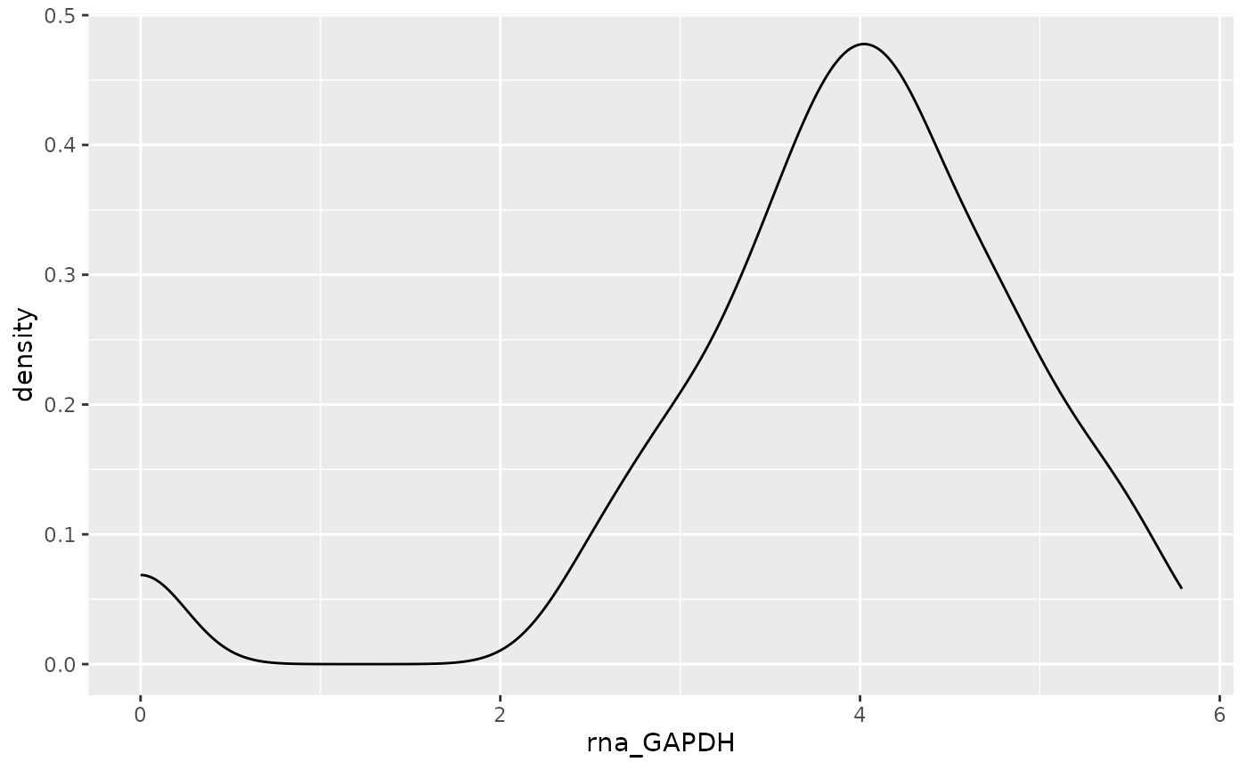
Next, we will add a fill attribute based on the metadata variable
entered. The metadata variable is supplied to the fill attribute, again
using .data[[]].
object <- AML_Seurat
feature <- "rna_GAPDH"
metadata <- "condensed_cell_type"

data <-
  fetch_data(
    object,
    # variables to fetch, the feature and metadata variable
    vars =
      c(feature,
        metadata
        )
    )

plot <- ggplot(
    data = data,
    aes(x = .data[[feature]], fill = .data[[metadata]])
    ) +
    geom_density()

plot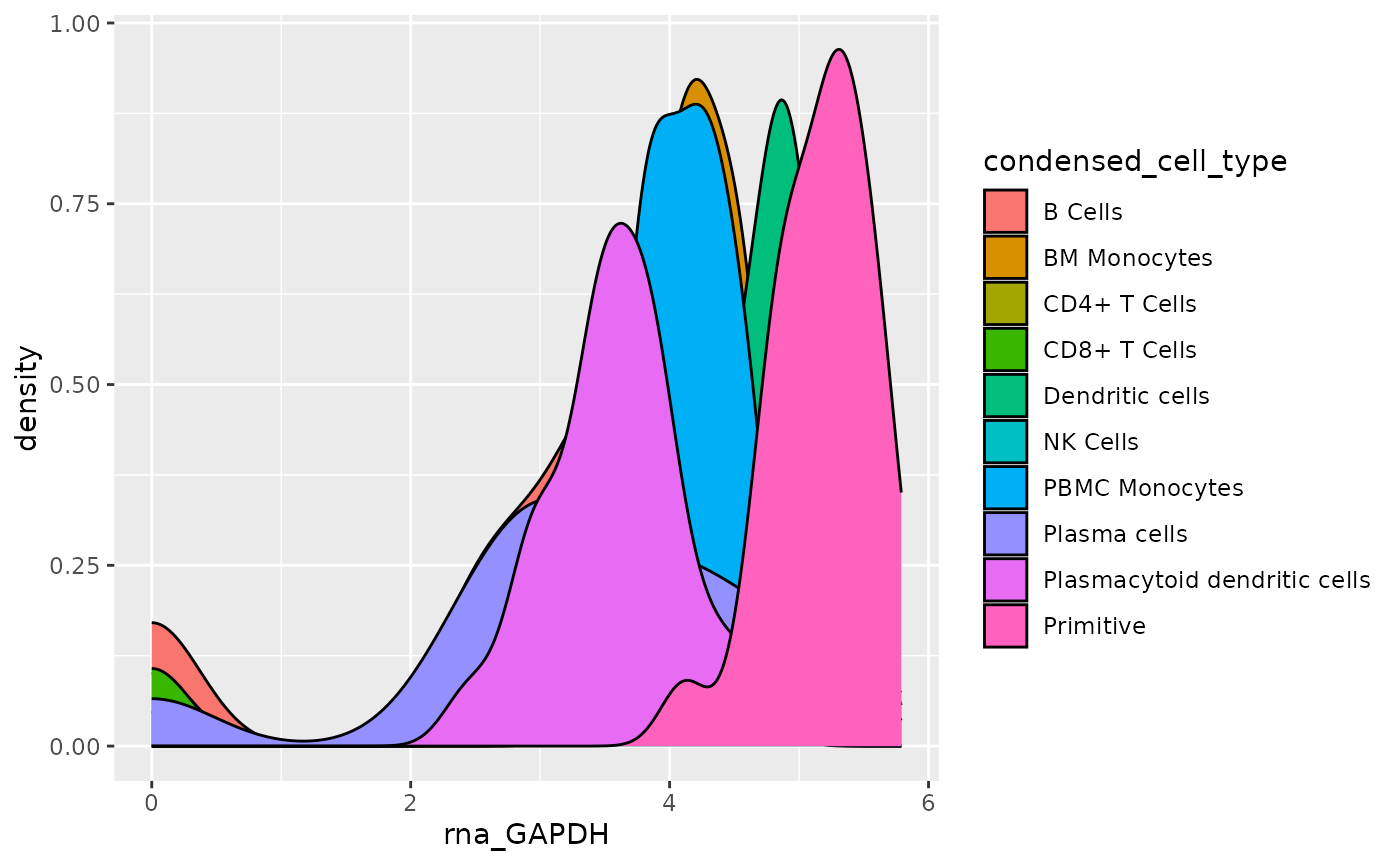
For this plot to be interperetable, the curves will need to be
“split” out into separate plots. This is done with
facet_wrap().
object <- AML_Seurat
feature <- "rna_GAPDH"
metadata <- "condensed_cell_type"

data <-
  fetch_data(
    object,
    # variables to fetch, the feature and metadata variable
    vars =
      c(feature,
        metadata
        )
    )

plot <- ggplot(
    data = data,
    aes(x = .data[[feature]], fill = .data[[metadata]])
    ) +
    geom_density() +
    ggplot2::facet_wrap(
        vars(.data[[metadata]]),
        # Set a two-column layout
        ncol = 2
    )

plot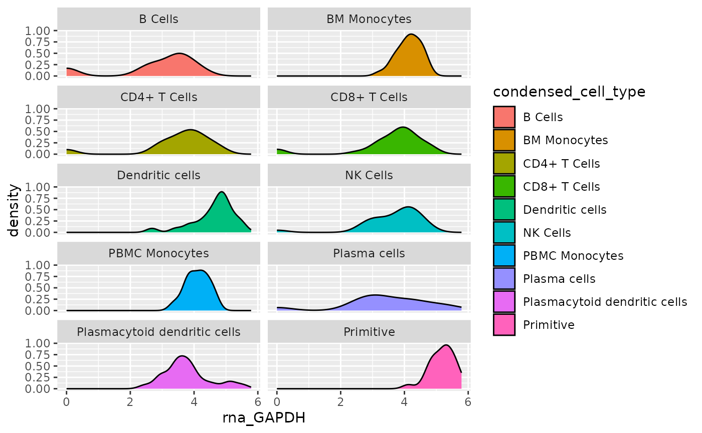
Next, plot visuals are improved. theme_cowplot() from
the cowplot package is applied. This removes grids from the
plot region, and adds axes on the left and bottom of the plot.
The following additional changes will be added with a custom theme:
- Labels for each facet are horizontally centered.
- The legend is removed from the plot.
- The gray box behind facet labels is made transparent using
strip.background = element_rect(fill = "#FFFFFF00"). The last two digits in the fill color “#FFFFFF00” make the background transparent by setting the alpha value of the hex code color to zero. - The text is made bold and shrank via
strip.text.
if (!require("cowplot", quietly = TRUE)){
  install.packages("cowplot")
}

library(cowplot)
object <- AML_Seurat
feature <- "rna_GAPDH"
metadata <- "condensed_cell_type"

data <-
  fetch_data(
    object,
    # variables to fetch, the feature and metadata variable
    vars =
      c(feature,
        metadata
        )
    )

plot <- ggplot(
    data = data,
    aes(x = .data[[feature]], fill = .data[[metadata]])
    ) +
    geom_density() +
    ggplot2::facet_wrap(
      vars(.data[[metadata]]),
      ncol = 2
      ) +
    cowplot::theme_cowplot() +
    theme(
      plot.title = element_text(hjust = 0.5),
      legend.position = "none",
      strip.background = element_rect(fill = "#FFFFFF00"),
      strip.text = element_text(face = "bold", size = rel(0.8))
      )

plot
At this point, the plot is in a finished form and is ready to be packaged in a function.
At this stage, simply transfer the variables defined at the beginning to the function as parameters, and move the subsequent code into the function.
# Transfer variables to parameters
# object <- AML_Seurat
# feature <- "rna_GAPDH"
# metadata <- "condensed_cell_type"
density_plot <-
function(
object,
feature,
metadata
){
data <-
fetch_data(
object,
# variables to fetch, the feature and metadata variable
vars =
c(feature,
metadata
)
)
plot <- ggplot(
data = data,
aes(x = .data[[feature]], fill = .data[[metadata]])
) +
geom_density() +
ggplot2::facet_wrap(
vars(.data[[metadata]]),
ncol = 2
) +
cowplot::theme_cowplot() +
theme(
plot.title = element_text(hjust = 0.5),
legend.position = "none",
strip.background = element_rect(fill = "#FFFFFF00"),
strip.text = element_text(face = "bold", size = rel(0.8))
)
plot
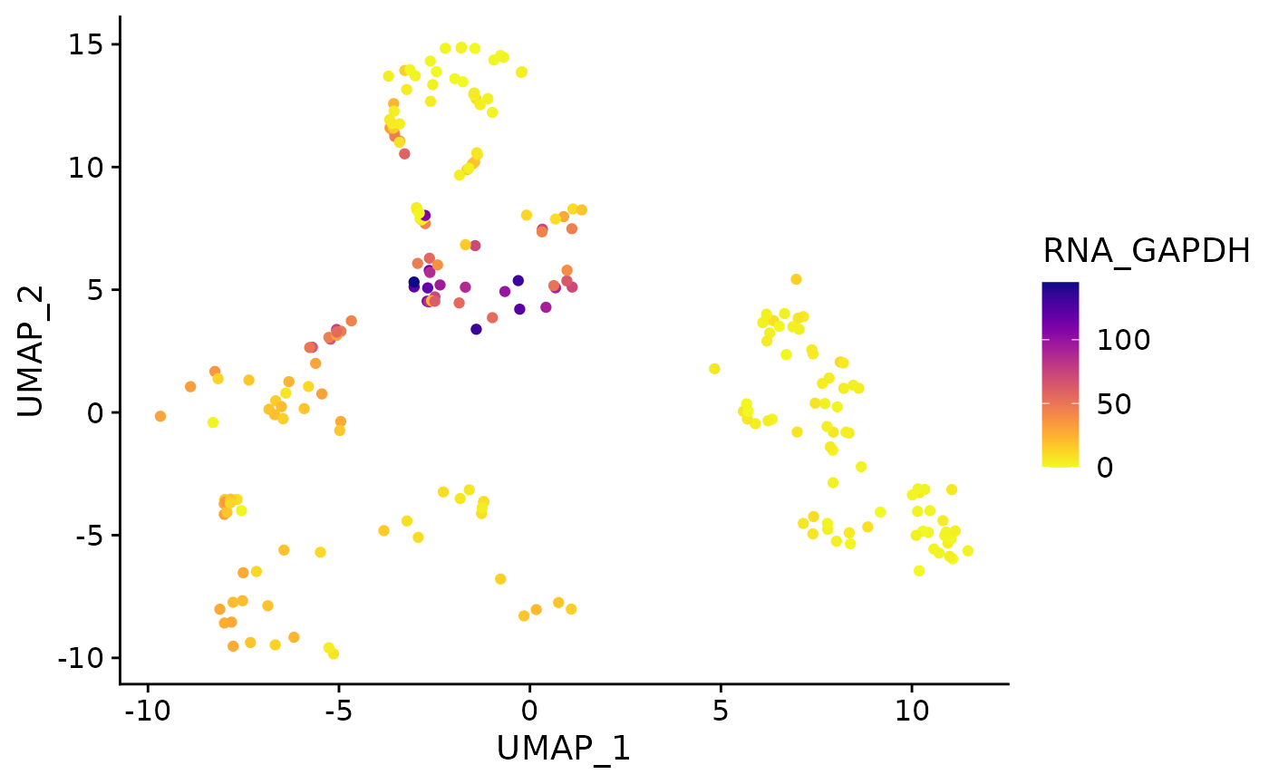
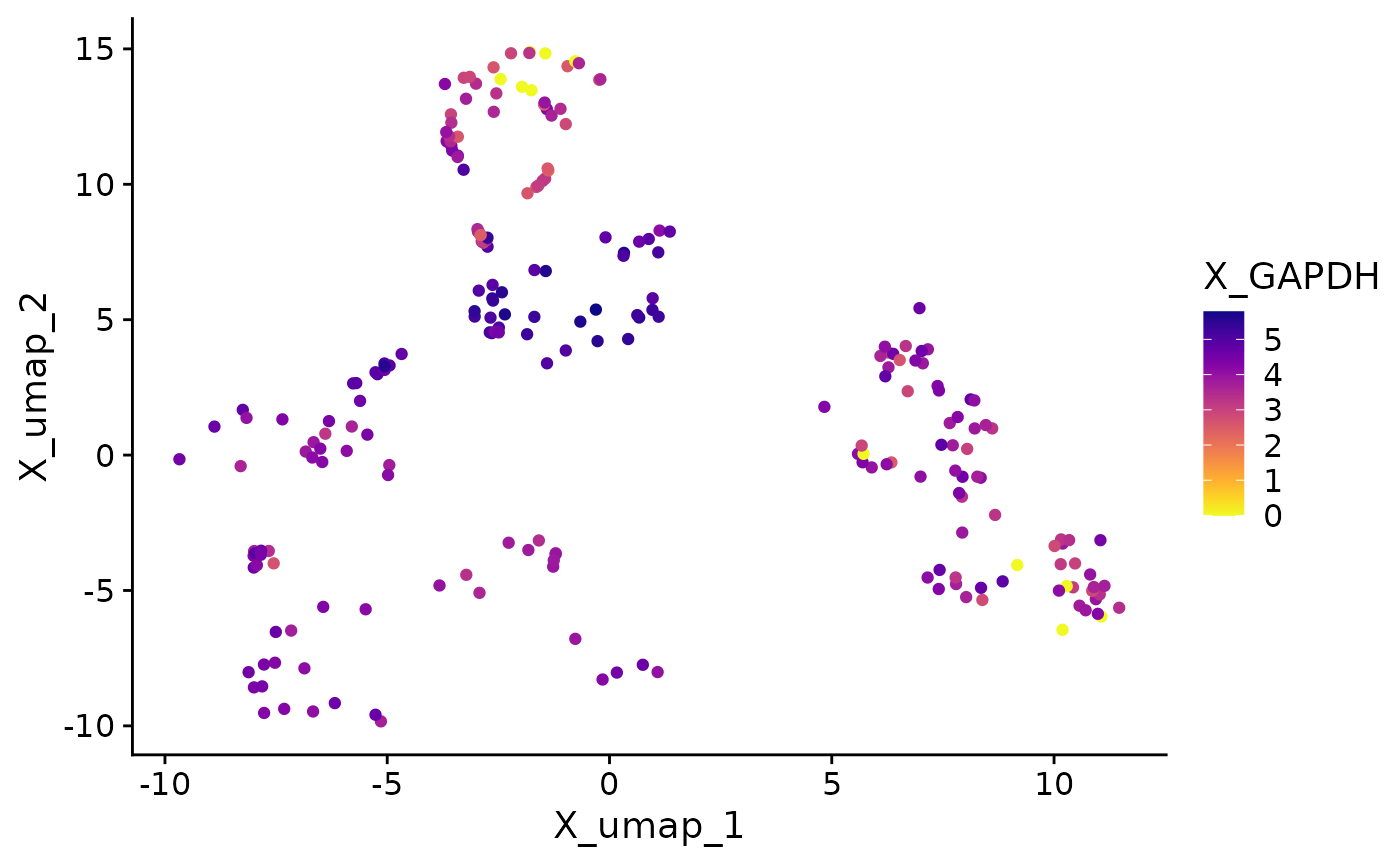
}Now we call the function on each supported object class. The plots have almost identical visuals, except for differences in assay names when entering features.


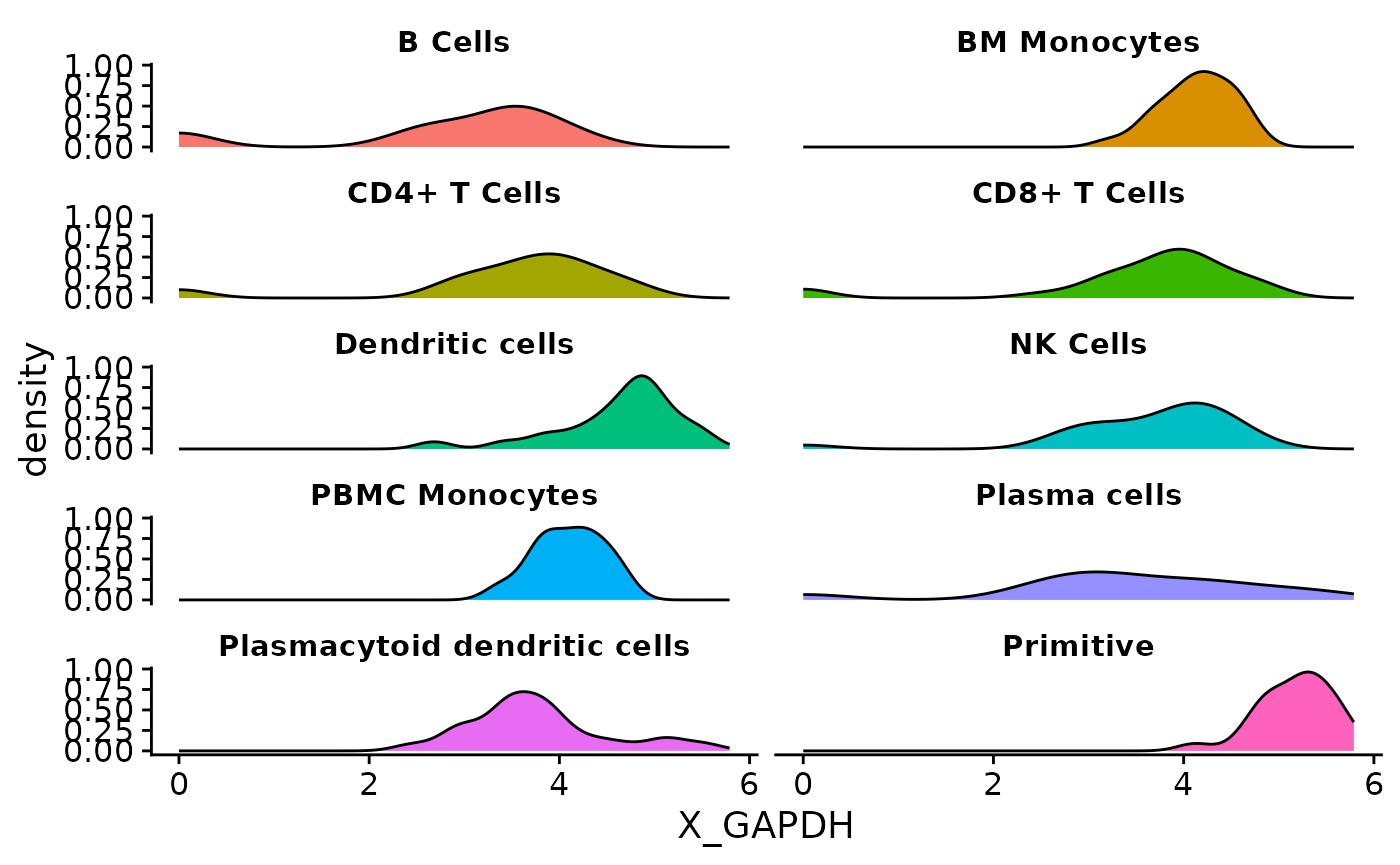
The process described here can be applied to the creation of any other single-cell visualization that uses expression data, metadata, or reduction coordinates. SCUBA facilitates data access in visualization functions, allowing users to access data through a call to an access function instead of doing object-specific data wrangling.
Utility Methods for Visualization Functions
SCUBA provides several utility methods for plotting functions that define default properties, allowing users to optionally specify reductions and layers to user for plotting without requiring users to enter these parameters.
Below is an example feature plot function that uses the following utility functions:
-
default_reduction(): Returns the key of a default reduction to use. -
default_layer(): Returns the conventional name of the normalized layer in the object. -
get_all_cells(): Returns the IDs of all cells in the object. -
reduction_dimnames(): Forms the names of reduction dimensions to pull, for passage tovarsinfetch_data.
feature_plot <-
function(
object,
feature,
dims = c(1, 2),
reduction = NULL,
layer = NULL,
cells = NULL
){
# Determine a default reduction if the user does not enter one
if (is.null(reduction)){
reduction <- default_reduction(object)
}
# Define a default layer if undefined
if (is.null(layer)){
layer <- default_layer(object)
}
# Cells: if undefined, set to all cells in object
if (is.null(cells)){
cells <- get_all_cells(object)
}
# Form syntax for pulling reduction coordinates using the reduction
# name and the dimensions entered in the function
reduction_vars <-
reduction_dimnames(
object = object,
reduction = reduction,
dims = dims
)
data <-
fetch_data(
object = object,
vars = c(reduction_vars, feature),
layer = layer,
cells = cells
)
plot <-
ggplot(
data,
aes(
x = .data[[reduction_vars[1]]],
y = .data[[reduction_vars[2]]],
color = .data[[feature]]
)
) +
geom_point() +
cowplot::theme_cowplot() +
scale_color_gradientn(
# Color cells using the viridis palette
colors = viridisLite::plasma(12, direction = -1)
) +
theme(
plot.title = element_text(hjust = 0.5),
strip.background = element_rect(fill = "#FFFFFF00"),
strip.text = element_text(face = "bold", size = rel(0.8))
)
plot
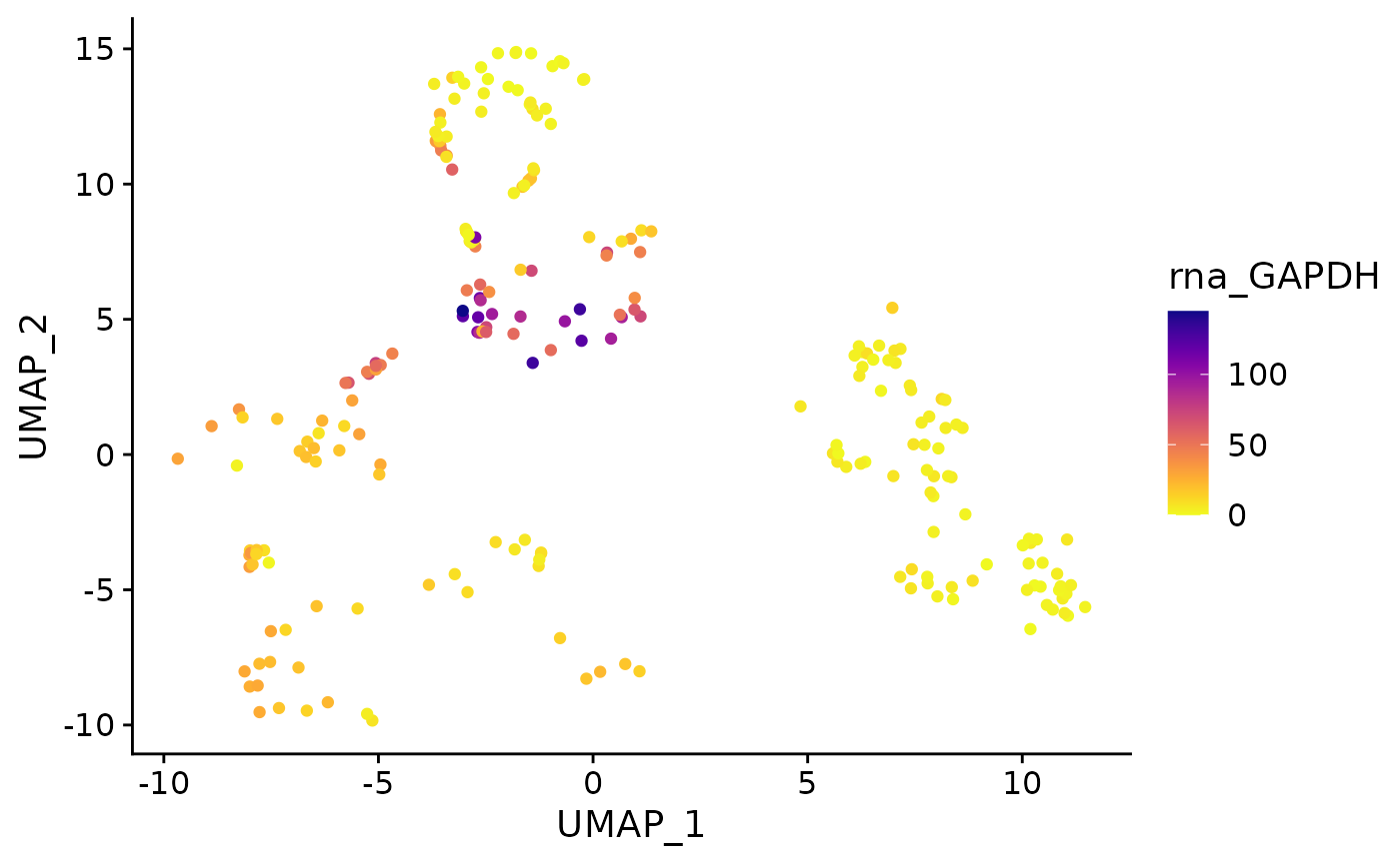
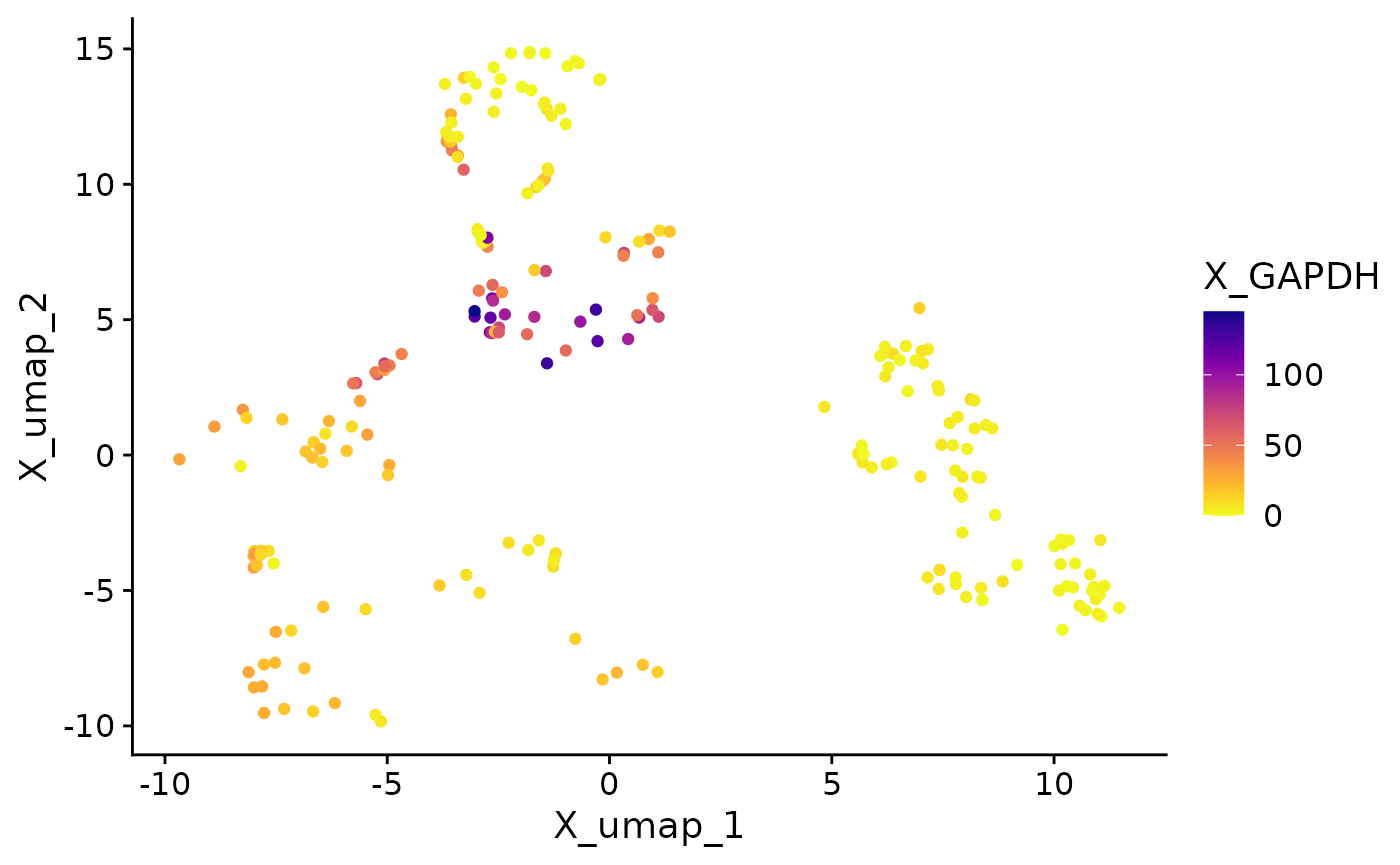
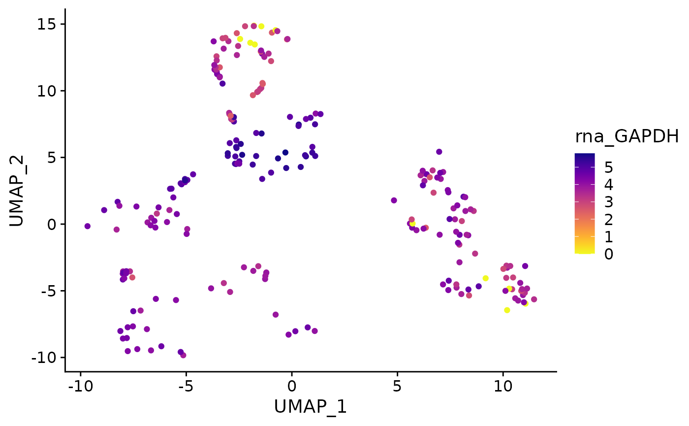
}Running function without specifying default reduction, layer: utility functions will supply defaults.
feature_plot(
  object = AML_Seurat,
  feature = "rna_GAPDH"
  )
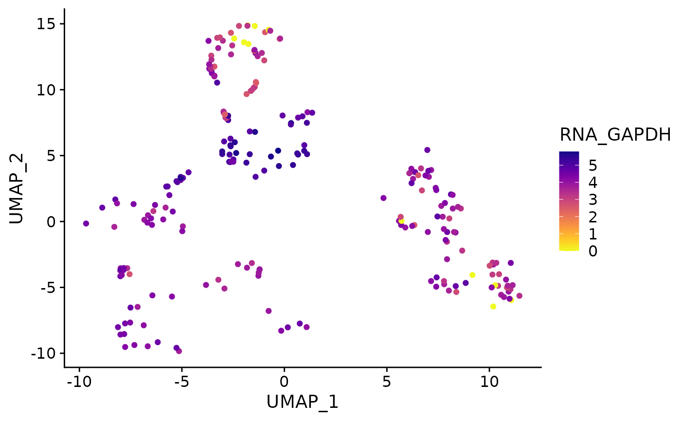
Running the function with the raw counts layer:
feature_plot(
  object = AML_Seurat,
  feature = "rna_GAPDH",
  layer = "counts"
  )